5 R

5.1 Assignment

For assigning a value to a variable, i use <- unless the variable is a parameter or an argument - then i use =:

variable <- "value"                                  # 1
                                                     # 2
name_of_function <- function(parameter = "value") {  # 3
                                                     # 4
}                                                    # 5

5.2 Debugging

5.2.1 Printing out a value

print(2)  # 1
## [1] 2

5.2.2 Datatype

For figuring out the datatype[56]:

class(2)  # 1
## [1] "numeric"

5.2.3 Datatype and value

str(2)  # 1
##  num 2

5.2.4 Is the value not set?

is.null(variable)  # 1
## [1] FALSE

5.2.5 Stopping execution

stop("error message")  # 1
                       # 2

5.3 Numbers

5.3.1 Converting a string to a number

number = "3"  # 1
str(number)   # 2
##  chr "3"
                                      # 1
numeric_number <- as.numeric(number)  # 2
str(numeric_number)                   # 3
##  num 3

5.3.2 Sequencing

seq(0, 14, 2)  # 1
## [1]  0  2  4  6  8 10 12 14

5.3.3 Rounding

5.3.3.1 Normal rounding

round(123.456, digits = 1)  # 1
## [1] 123.5
round(122.5)  # 1
## [1] 122
round(123.5)  # 1
## [1] 124

5.3.3.2 Significant digits

For printing only significant digits, there’s the function signif which takes two parameters: the initial number x and the number of significant digits digits:

number <- 123.456                                                 # 1
                                                                  # 2
number_with_significant_digits <- signif(x = number, digits = 4)  # 3
print(number_with_significant_digits)                             # 4
## [1] 123.5

5.3.3.3 Prefixes

For formatting with prefixes, one can use the function format_SI[57] from the package BAAQMD/strtools[58]:

number <- c(1234.56, 0.123456)  # 1
librarian::shelf(c(             # 2
  "strtools"                    # 3
))                              # 4
format_SI(number)               # 5
## [1] "1k"   "123m"
format_SI(number, fixed=TRUE)  # 1
## [1] "1k" "0k"
format_SI(number, engineering=TRUE)  # 1
## [1] "1.234560000k" "0.000123456k"
format_SI(number, digits=2)  # 1
## [1] "1.23k"   "123.46m"

5.3.3.4 Powers and units

For using powers and units, there is the package formatdown[59]:

librarian::shelf(c(                            # 1
  "formatdown"                                 # 2
))                                             # 3
numbers <- c(123.456, 2e-6, 5e8, 0.23)         # 4
format_power_numbers <- format_power(numbers)  # 5
## Warning in format_power(numbers): `format_power()` is deprecated. Use `format_numbers()`
##               which offers additional arguments and access to package options.
format_power_numbers_digits <- format_power(numbers, digits = 2)  # 1
## Warning in format_power(numbers, digits = 2): `format_power()` is deprecated. Use `format_numbers()`
##               which offers additional arguments and access to package options.
format_power_numbers_sci <- format_power(numbers, format="sci")  # 1
## Warning in format_power(numbers, format = "sci"): `format_power()` is deprecated. Use `format_numbers()`
##               which offers additional arguments and access to package options.
format_power_numbers_omit <- format_power(numbers, omit_power = c(-6, -6))  # 1
## Warning in format_power(numbers, omit_power = c(-6, -6)): `format_power()` is deprecated. Use `format_numbers()`
##               which offers additional arguments and access to package options.
format_power_numbers_set <- format_power(numbers, set_power = 5)  # 1
## Warning in format_power(numbers, set_power = 5): `format_power()` is deprecated. Use `format_numbers()`
##               which offers additional arguments and access to package options.
units(numbers) <- "kg m-3"                                     # 1
format_units_numbers <- format_units(x=numbers, unit="g l-1")  # 2
## Warning in format_units(x = numbers, unit = "g l-1"): `format_units()` is deprecated. Use `format_numbers()`
##               which offers additional arguments and access to package options.

\(\small 123.5\), \(\small 2.000 \times 10^{-6}\), \(\small 500.0 \times 10^{6}\), \(\small 0.2300\)

\(\small 120\), \(\small 2.0 \times 10^{-6}\), \(\small 500 \times 10^{6}\), \(\small 0.23\)

\(\small 123.5\), \(\small 2.000 \times 10^{-6}\), \(\small 5.000 \times 10^{8}\), \(\small 0.2300\)

\(\small 123.5 \times 10^{0}\), \(\small 0.000002000\), \(\small 500.0 \times 10^{6}\), \(\small 230.0 \times 10^{-3}\)

\(\small 123.5\), \(\small 0.00000000002000 \times 10^{5}\), \(\small 5000 \times 10^{5}\), \(\small 0.2300\)

123.456000 [g/L], 0.000002 [g/L], 500000000.000000 [g/L], 0.230000 [g/L]

5.4 Time

5.4.1 Converting to time

string_of_time = "2020.7.08 16:43:59"  # 1
str(string_of_time)                    # 2
##  chr "2020.7.08 16:43:59"
                                                                                                                       # 1
librarian::shelf(c(                                                                                                    # 2
  "lubridate"                                                                                                          # 3
))                                                                                                                     # 4
                                                                                                                       # 5
string_of_time_as_time <- parse_date_time(string_of_time, c("%Y.%m.%d %H:%M", "%m.%d.%Y %H:%M", "%Y.%m.%d %H:%M:%S"))  # 6
str(string_of_time_as_time)                                                                                            # 7
##  POSIXct[1:1], format: "2020-07-08 16:43:59"

[60].

5.4.2 Parts of time

For ms, the package lubridate is needed. This function extracts the minutes and seconds.

time <- "2:53"           # 1
parsed_time <- ms(time)  # 2
print(parsed_time)       # 3
## [1] "2M 53S"

The time in the last minute is \(\qty{53}{\s}\).

s <- as.numeric(parsed_time)  # 1

The time is \(\qty{173}{\s}\).

5.5 Array

5.5.1 Creation

An array can be created using the function c:

array <- c("value_1", "value_2")  # 1
print(array)                      # 2
## [1] "value_1" "value_2"

5.5.2 Referencing position

Referencing a position inside the array takes place using brackets whereas the first position has the index 1:

value_at_position_2 <- array[2]  # 1
print(value_at_position_2)       # 2
## [1] "value_2"
                       # 1
array[2] <- "value_3"  # 2
print(array)           # 3
## [1] "value_1" "value_3"

5.5.3 Multidimensional

Arrays with the same length can be connected into data.frame:

array_2 <- c("value_3", "value_4")        # 1
data_frame <- data.frame(array, array_2)  # 2
print(data_frame)                         # 3
##     array array_2
## 1 value_1 value_3
## 2 value_3 value_4

5.5.4 Column names

A data.frame can have column names:

colnames(data_frame) <- c(  # 1
  "array",                  # 2
  "array 2"                 # 3
)                           # 4
                            # 5
print(data_frame)           # 6
##     array array 2
## 1 value_1 value_3
## 2 value_3 value_4

5.5.5 Adding column[61]

data_frame_with_array_2 <- cbind(data_frame, array_2)  # 1
                                                       # 2
print(data_frame_with_array_2)                         # 3
##     array array 2 array_2
## 1 value_1 value_3 value_3
## 2 value_3 value_4 value_4

5.5.6 Row names

rownames(data_frame) <- c(  # 1
  "Caption of first row",   # 2
  "Caption of second row"   # 3
)                           # 4
                            # 5
print(data_frame)           # 6
##                         array array 2
## Caption of first row  value_1 value_3
## Caption of second row value_3 value_4

5.5.7 Importing data

Data can be imported from a text file into a data frame:

CO2_in_air <- read.table("co2_brw_surface-insitu_1_ccgg_DailyData.txt", header = TRUE, sep = "", dec = ".")  # 1
                                                                                                             # 2

Data can also be imported from a comma-separated-values-(CSV-)file into a data frame:

washing_cycles <- read.table("washing-cycles.csv", header = TRUE, sep = ",", dec = ".")  # 1

5.5.8 Printing first rows

print(head(washing_cycles))  # 1
##              Algus Kestus Temperatuur Pöördeid.min      Kava Veenäit.enne
## 1 2018.12.24 19:05   0:29          40         1000  lühikava           NA
## 2 2018.12.24 23:03   0:29          30         1000  lühikava           NA
## 3  2018.12.24 0:27   1:54          40         1000  segakiud           NA
## 4 2018.12.26 14:30   0:47          30          800  käsipesu           NA
## 5 2018.12.26 23:35   0:47          40          800 villapesu           NA
## 6  2018.12.27 0:58   0:29          30         1000  lühikava      279.396
##   Veenäit.pärast Veekulu..l. kWh
## 1                         NA 0.5
## 2                         NA 0.2
## 3                         NA 0.4
## 4                         NA 0.4
## 5                         NA 0.4
## 6        279.428         3.2 0.3

5.5.9 Editing the look of a cell

librarian::shelf("kableExtra")                              # 1
coloured_cell <- cell_spec(data_frame[, 2], color = "red")  # 2

[62].

5.5.10 Editing the content

librarian::shelf("dplyr")                  # 1
mutate(data_frame, "array 2" = "mutated")  # 2
##                         array array 2
## Caption of first row  value_1 mutated
## Caption of second row value_3 mutated

[63].

5.5.11 Size

length(data_frame)  # 1
## [1] 2
                  # 1
nrow(data_frame)  # 2
## [1] 2

5.5.12 Looping

                                       # 1
for (index in 1:length(data_frame)) {  # 2
  print(data_frame[index])             # 3
}                                      # 4
##                         array
## Caption of first row  value_1
## Caption of second row value_3
##                       array 2
## Caption of first row  value_3
## Caption of second row value_4

5.5.13 Referencing by column name

print(data_frame$`array 2`)  # 1
## [1] "value_3" "value_4"

[64].

5.5.14 Subsetting

As washing_cycles also contains records with missing data i want them removed:

                                                                                                                                                     # 1
washing_cycles_with_full_records <- subset(washing_cycles, !is.na(`Veenäit.enne`) & "" != `Veenäit.pärast` & !is.na(`Veekulu..l.`) & !is.na(`kWh`))  # 2
                                                                                                                                                     # 3
print(head(washing_cycles_with_full_records))                                                                                                        # 4
##               Algus Kestus Temperatuur Pöördeid.min       Kava Veenäit.enne
## 6   2018.12.27 0:58   0:29          30         1000   lühikava      279.396
## 7  2018.12.27 19:32   0:44          30         1000   lühikava      279.439
## 9   2019.1.12 15:13   1:54          30         1000 sünteetika      280.071
## 10   2019.2.7 12:46   0:29          30         1000   lühikava      281.189
## 11  2019.2.16 21:56   0:29          30         1000   lühikava      281.522
## 12  2019.2.20 17:10   0:47          40          800  villapesu      281.698
##        Veenäit.pärast Veekulu..l. kWh
## 6             279.428         3.2 0.3
## 7             279.459         2.0 0.1
## 9  280.13400000000001         6.3 1.5
## 10 281.21499999999997         2.6 0.4
## 11 281.54899999999998         2.7 0.3
## 12            281.745         4.7 0.9

[65].

This was how to remove incomplete records by manually setting the columns that contain empty records. There is a move convenient method to do that without specifying columns:

washing_cycles_with_full_records <- washing_cycles[complete.cases(washing_cycles), ]  # 1

[64].

I only want to see the data in the column Kava:

program_in_washing_cycles <- subset(washing_cycles_with_full_records, select = `Kava`)  # 1
                                                                                        # 2
print(head(program_in_washing_cycles))                                                  # 3
##          Kava
## 6    lühikava
## 7    lühikava
## 9  sünteetika
## 10   lühikava
## 11   lühikava
## 12  villapesu

I only want to see cycles from the rows 2 to 4 in the second column:

print(washing_cycles_with_full_records[2:4, 2])  # 1
## [1] "0:44" "1:54" "0:29"

I want the last 216 rows to be removed:

number_of_rows_in_washing_cycles_with_full_records <- nrow(washing_cycles_with_full_records)                            # 1
data_frame_of_washing_cycles_with_full_records_without_last_records <- washing_cycles_with_full_records[                # 2
  -c((number_of_rows_in_washing_cycles_with_full_records - 215):number_of_rows_in_washing_cycles_with_full_records), ]  # 3
print(data_frame_of_washing_cycles_with_full_records_without_last_records)                                              # 4
##              Algus Kestus Temperatuur Pöördeid.min       Kava Veenäit.enne
## 6  2018.12.27 0:58   0:29          30         1000   lühikava      279.396
## 7 2018.12.27 19:32   0:44          30         1000   lühikava      279.439
## 9  2019.1.12 15:13   1:54          30         1000 sünteetika      280.071
##       Veenäit.pärast Veekulu..l. kWh
## 6            279.428         3.2 0.3
## 7            279.459         2.0 0.1
## 9 280.13400000000001         6.3 1.5

I only want to see hot cycles:

hot_cycles <- subset(washing_cycles_with_full_records, `Temperatuur` > 40)  # 1
print(hot_cycles)                                                           # 2
##                   Algus  Kestus Temperatuur Pöördeid.min                   Kava
## 23      2019.4.19 15:13    2:10          60         1000                  beebi
## 34       2019.7.6 16:05    1:54          60         1000             sünteetika
## 38      2019.7.10 13:30    1:54          60         1000               segakiud
## 65      2019.9.28 19:41    1:54          60         1000     segakiud, hygiene+
## 68      2019.9.29 16:39    2:10          90          400              autoclean
## 184 2020.11.15 19:19:59 1:54:59          60         1000     segakiud, hygiene+
## 203  2021.2.12 19:09:59 2:49:00          90         1300             Kochwäsche
## 206  2021.2.16 18:31:59 1:54:59          60         1000  sünteetika + hygiene+
## 320 11.12.2021 15:24:59 1:54:59          60         1000         segu, hygiene+
## 340 12.10.2021 23:22:00 2:49:00          90         1300    keedupesu, hygiene+
## 393  3.20.2022 14:42:00 2:59:00          90         1300 keedupesu, lisaloputus
## 425  6.24.2022 14:10:59 4:00:59          60         1300   puuvill, lisaloputus
## 427  6.24.2022 17:48:59 2:04:00          60         1000      segu, lisaloputus
## 439  7.17.2022 15:33:00 2:59:00          90          400              keedupesu
##     Veenäit.enne     Veenäit.pärast Veekulu..l. kWh
## 23       284.498 284.53699999999998         3.9 2.3
## 34       287.732 287.80200000000002         7.0 1.0
## 38       288.129 288.20600000000002         7.7 2.3
## 65       292.237 292.30799999999999         7.1 0.9
## 68       292.478 292.49799999999999         2.0 0.5
## 184      316.293 316.31200000000001         1.9 0.4
## 203      321.112 321.17500000000001         6.3 3.7
## 206      321.487 321.52199999999999         3.5 0.6
## 320      341.609 341.67599999999999         6.7 0.9
## 340      344.372 344.41000000000003         3.8 1.2
## 393      352.388 352.42599999999999         3.8 0.9
## 425      358.710 358.73599999999999         2.6 1.4
## 427      358.805 358.82999999999998         2.5 0.4
## 439      360.281             360.31         2.9 0.9

I only want to see the indices of the cycles at the temperature of \(313.15 \times \mathrm{K}\):

which(washing_cycles_with_full_records[3] == 40)  # 1
##  [1]   6   9  13  14  16  18  23  25  29  38  44  48  52  56  66  73  80  89  91
## [20]  93  98 102 112 113 118 120 123 126 150 153 162 167 169 172 174 176 180 181
## [39] 182 186 187 191 193 197 198 202 203 206 207 208 212 214 215 217

5.5.15 Sorting

Displaying the indices of the descending sorted values of a vector:

librarian::shelf("dplyr")                                                         # 1
desc(as.matrix(subset(head(washing_cycles_with_full_records), select = `Kava`)))  # 2
## [1] -1 -1 -5 -1 -1 -6

[66(pp. 7, 21)].

Sorting values in ascending order according to the program:

head(arrange(washing_cycles_with_full_records, `Kava`))  # 1
##                 Algus  Kestus Temperatuur Pöördeid.min                Kava
## 1  2021.2.12 19:09:59 2:49:00          90         1300          Kochwäsche
## 2  7.13.2022 18:17:59 0:59:00          30          800            Trainers
## 3     2019.9.29 16:39    2:10          90          400           autoclean
## 4     2019.4.19 15:13    2:10          60         1000               beebi
## 5  7.17.2022 15:33:00 2:59:00          90          400           keedupesu
## 6 12.10.2021 23:22:00 2:49:00          90         1300 keedupesu, hygiene+
##   Veenäit.enne     Veenäit.pärast Veekulu..l. kWh
## 1      321.112 321.17500000000001         6.3 3.7
## 2      359.990            360.005         1.5 0.2
## 3      292.478 292.49799999999999         2.0 0.5
## 4      284.498 284.53699999999998         3.9 2.3
## 5      360.281             360.31         2.9 0.9
## 6      344.372 344.41000000000003         3.8 1.2

5.5.16 Totals

librarian::shelf("janitor")                                                                                                                                                           # 1
adorn_totals(dat = head(subset(x = washing_cycles_with_full_records, select = c(`Algus`, `Veekulu..l.`))), where = "row", fill = "", na.rm = TRUE, name = "Kokku", c(`Veekulu..l.`))  # 2
##             Algus Veekulu..l.
##   2018.12.27 0:58         3.2
##  2018.12.27 19:32         2.0
##   2019.1.12 15:13         6.3
##    2019.2.7 12:46         2.6
##   2019.2.16 21:56         2.7
##   2019.2.20 17:10         4.7
##             Kokku        21.5

[67].

5.5.17 Mean

Mean row-wise can be calculated using rowMeans()[68].

t_1 <- c(7.508, 4.452, 3.434, 2.978, 2.752)       # 1
t_2 <- c(7.775, 4.515, 3.434, 2.978, 2.752)       # 2
t_3 <- c(7.685, 4.47, 3.603, 2.992, 2.732)        # 3
                                                  # 4
data_frame_of_mass_time <- data.frame(            # 5
  t_1,                                            # 6
  t_2,                                            # 7
  t_3                                             # 8
)                                                 # 9
                                                 # 10
rowMeans(x = data_frame_of_mass_time[, c(1:3)])  # 11
## [1] 7.656000 4.479000 3.490333 2.982667 2.745333

5.6 Functions

Functions can be made using the keyword function:

add <- function(first, second, digits = 2) {                           # 1
  return(signif(first + second, digits = digits))                      # 2
}                                                                      # 3
                                                                       # 4
add(first = 123, second = 456) # using the default value 2 for digits  # 5
## [1] 580
                                                   # 1
sum <- add(first = 123, second = 456, digits = 1)  # 2

It is not possible to assign an argument with the same name as the parameter[69]. In the example above, the value for first could not be first although there might be an external variable first, id est first = first is not allowed. I have to use different names.

5.7 Square root

A square root can be calculated using the function sqrt():

input_for_square_root <- 4                  # 1
square_root <- sqrt(input_for_square_root)  # 2

The square root of \(\num{4}\) is \(\num{2}\).

5.8 Derivation

initial_function <- "x^3 + x^2"                  # 1
functionToUse <- parse(text = initial_function)  # 2
                                                 # 3
librarian::shelf(c(                              # 4
  "Ryacas"                                       # 5
))                                               # 6
                                                 # 7
derivative = D(functionToUse, "x")               # 8
string_of_derivative <- deparse(derivative)      # 9

The derivative of \(x^3 + x^2\) is \(3 * x^2 + 2 * x\).

equality <- paste(string_of_derivative, "== 0")  # 1
print(equality)                                  # 2
## [1] "3 * x^2 + 2 * x == 0"
print(paste("Solve(", equality, ", x)", sep = ""))  # 1
## [1] "Solve(3 * x^2 + 2 * x == 0, x)"
print(y_rmvars(paste("Solve(", equality, ", x)", sep = "")))  # 1
## [1] "((Solve(3 * x^2 + 2 * x == 0, x)) /:: { _lhs == _rhs <- rhs })"
critical_places <- yac_str(y_rmvars(paste("Solve(", equality, ", x)", sep = "")))  # 1
print(critical_places)                                                             # 2
## [1] "{0,(-2)/3}"
critical_places_as_r <- as_r(critical_places)  # 1
print(critical_places_as_r)                    # 2
## [1] "0"      "(-2)/3"
critical_solution_1 <- (critical_places_as_r[1])  # 1
critical_solution_2 <- critical_places_as_r[2]    # 2

The critical solutions of \(x^3 + x^2\) are 0 and (-2)/3.

5.9 Comments

Comments can be done with #:

print(sum) # printing out the value of sum  # 1
## [1] 600

5.10 Strings

Strings can be written using either apostrophes or quotation marks.

For substituting something inside a string, gsub can be used[70]:

gsub("_", "\\_", array, fixed = TRUE)  # 1
## [1] "value\\_1" "value\\_3"

Here, in order to preserve a backslash, it has to be escaped as otherwise, it escapes the underscore. If I would turn off fixed, the function would work like with regular expressions.

5.11 Branching

ifelse(is.na(NA), "Not Available", "Available")  # 1
## [1] "Not Available"

5.12 Table

5.12.1 A user-friendly look

A table that is not just in R code but designed and all can be created using kable and kableExtra[71]. I have built a wrapper function print_table for that purpose so that I do not have to rewrite some general things from table to table. An example table is 5.1 on the page .

omega <- c(932.0058, 827.2861, 733.0383, 628.3185, 523.5988, 418.8790, 314.1593)                  # 1
omega_P <- c(0.03966657, 0.04155546, 0.05073632, 0.05411874, 0.05817764, 0.03878509, 0.01811760)  # 2
                                                                                                  # 3
data_frame_of_precession <- data.frame(                                                           # 4
  omega,                                                                                          # 5
  omega_P                                                                                         # 6
)                                                                                                 # 7
                                                                                                  # 8
colnames(data_frame_of_precession) <- c(                                                          # 9
  "$\\frac{\\omega}{\\unit{\\per\\s}}$",                                                         # 10
  "$\\frac{\\omega_\\text{P}}{\\unit{\\per\\s}}$"                                                # 11
)                                                                                                # 12
                                                                                                 # 13
print_table(                                                                                     # 14
  table = data_frame_of_precession,                                                              # 15
  caption = "Pretsessiooni nurkkiiruse sõltuvus güroskoobi nurkkiirusest."                       # 16
)                                                                                                # 17
Table 5.1: Table 5.2: Pretsessiooni nurkkiiruse sõltuvus güroskoobi nurkkiirusest.
\(\frac{\omega}{\unit{\per\s}}\) \(\frac{\omega_\text{P}}{\unit{\per\s}}\)
932.01 0.04
827.29 0.04
733.04 0.05
628.32 0.05
523.60 0.06
418.88 0.04
314.16 0.02

5.12.2 Untolerated symbols

I have to pay attention that there can’t be any underscores inside the table unless they are part of an equation. They can be escaped using gsub and the result is shown as the table 5.3 on the page .

print_table(                                                                          # 1
  table = sapply(data_frame, function(value) gsub("_", "\\_", value, fixed = TRUE)),  # 2
  caption = "Caption."                                                                # 3
)                                                                                     # 4
Table 5.3: Table 5.4: Caption.
array array 2
value_1 value_3
value_3 value_4

Inside the table, backslashes must be escaped.

5.12.3 Number of digits after comma

Tables 5.5 on the page and 5.7 on the page are for comparing the number of digits after comma. The table 5.5 has the default number of digits and the table 5.7 has another number of digits in every number after comma.

water_report <- head(subset(x = washing_cycles_with_full_records, select = c(`Algus`, `Veenäit.enne`, `Veenäit.pärast`)))  # 1
                                                                                                                           # 2
librarian::shelf(c(                                                                                                        # 3
  'dplyr'                                                                                                                  # 4
))                                                                                                                         # 5
                                                                                                                           # 6
water_report <- water_report %>%                                                                                           # 7
  mutate(`Veenäit.pärast` = as.numeric(`Veenäit.pärast`))                                                                  # 8
                                                                                                                           # 9
colnames(water_report) <- c(                                                                                              # 10
  "Start",                                                                                                                # 11
  "$\\mathrm{\\frac{\\text{Used water before}}{\\mathrm{m^3}}}$",                                                         # 12
  "$\\mathrm{\\frac{\\text{Used water after}}{\\mathrm{m^3}}}$"                                                           # 13
)                                                                                                                         # 14
                                                                                                                          # 15
print_table(                                                                                                              # 16
  table = water_report,                                                                                                   # 17
  caption = "Water report with numbers with up to two digits after comma."                                                # 18
)                                                                                                                         # 19
Table 5.5: Table 5.6: Water report with numbers with up to two digits after comma.
Start \(\mathrm{\frac{\text{Used water before}}{\mathrm{m^3}}}\) \(\mathrm{\frac{\text{Used water after}}{\mathrm{m^3}}}\)
6 2018.12.27 0:58 279.40 279.43
7 2018.12.27 19:32 279.44 279.46
9 2019.1.12 15:13 280.07 280.13
10 2019.2.7 12:46 281.19 281.21
11 2019.2.16 21:56 281.52 281.55
12 2019.2.20 17:10 281.70 281.74

[66(p. 38) to 42].

print_table(                                                                  # 1
  table = water_report,                                                       # 2
  caption = "Water report with numbers with up to four digits after comma.",  # 3
  digits = 4                                                                  # 4
)                                                                             # 5
Table 5.7: Table 5.8: Water report with numbers with up to four digits after comma.
Start \(\mathrm{\frac{\text{Used water before}}{\mathrm{m^3}}}\) \(\mathrm{\frac{\text{Used water after}}{\mathrm{m^3}}}\)
6 2018.12.27 0:58 279.396 279.428
7 2018.12.27 19:32 279.439 279.459
9 2019.1.12 15:13 280.071 280.134
10 2019.2.7 12:46 281.189 281.215
11 2019.2.16 21:56 281.522 281.549
12 2019.2.20 17:10 281.698 281.745

5.12.4 Additional header

It’s also possible for the table to have an additional header whose columns span over multiple columns in the first header[72] (the table 5.9 on the page ):

print_table(                                         # 1
  table = water_report,                              # 2
  caption = "Water report with additional header.",  # 3
  additional_header = c("Spanned header" = 4)        # 4
)                                                    # 5
Table 5.9: Table 5.10: Water report with additional header.
Spanned header
Start \(\mathrm{\frac{\text{Used water before}}{\mathrm{m^3}}}\) \(\mathrm{\frac{\text{Used water after}}{\mathrm{m^3}}}\)
6 2018.12.27 0:58 279.40 279.43
7 2018.12.27 19:32 279.44 279.46
9 2019.1.12 15:13 280.07 280.13
10 2019.2.7 12:46 281.19 281.21
11 2019.2.16 21:56 281.52 281.55
12 2019.2.20 17:10 281.70 281.74

5.12.5 Look

It’s possible to change the look of a row (the table 5.11 on the page ):

print_table(                                   # 1
  table = water_report,                        # 2
  caption = "Water report with coloured row."  # 3
) %>%                                          # 4
  row_spec(2, color = "teal")                  # 5
Table 5.11: Table 5.12: Water report with coloured row.
Start \(\mathrm{\frac{\text{Used water before}}{\mathrm{m^3}}}\) \(\mathrm{\frac{\text{Used water after}}{\mathrm{m^3}}}\)
6 2018.12.27 0:58 279.40 279.43
7 2018.12.27 19:32 279.44 279.46
9 2019.1.12 15:13 280.07 280.13
10 2019.2.7 12:46 281.19 281.21
11 2019.2.16 21:56 281.52 281.55
12 2019.2.20 17:10 281.70 281.74

Here, %>% means piping.

And it’s possible to change the look of a column (the table 5.13 on the page ):

print_table(                                   # 1
  table = water_report,                        # 2
  caption = "Water report with wider column."  # 3
) %>%                                          # 4
  column_spec(1, width = "16em")               # 5
Table 5.13: Table 5.14: Water report with wider column.
Start \(\mathrm{\frac{\text{Used water before}}{\mathrm{m^3}}}\) \(\mathrm{\frac{\text{Used water after}}{\mathrm{m^3}}}\)
6 2018.12.27 0:58 279.40 279.43
7 2018.12.27 19:32 279.44 279.46
9 2019.1.12 15:13 280.07 280.13
10 2019.2.7 12:46 281.19 281.21
11 2019.2.16 21:56 281.52 281.55
12 2019.2.20 17:10 281.70 281.74

5.12.6 Landscape

If the table is too wide to fit the portrait format, it can be displayed in the landscape mode (the table 5.15 on the page ):

print_table(                              # 1
  table = water_report,                   # 2
  caption = "Water report as landscape."  # 3
) %>%                                     # 4
  landscape()                             # 5
Table 5.15: Table 5.16: Water report as landscape.
Start \(\mathrm{\frac{\text{Used water before}}{\mathrm{m^3}}}\) \(\mathrm{\frac{\text{Used water after}}{\mathrm{m^3}}}\)
6 2018.12.27 0:58 279.40 279.43
7 2018.12.27 19:32 279.44 279.46
9 2019.1.12 15:13 280.07 280.13
10 2019.2.7 12:46 281.19 281.21
11 2019.2.16 21:56 281.52 281.55
12 2019.2.20 17:10 281.70 281.74

5.12.7 Footnotes

Linked footnotes don’t work with kable. Footnotes can be created like this (the table 5.17 on the page ):

                                                                 # 1
DATA_FRAME_OF_COMPARISON <- data.frame(                          # 2
  0.3                                                            # 3
)                                                                # 4
                                                                 # 5
colnames(DATA_FRAME_OF_COMPARISON) <- c(                         # 6
  paste("$\\frac{T_\\text{dew}}{}$", footnote_marker_number(1))  # 7
)                                                                # 8
                                                                 # 9
print_table(                                                    # 10
  table = DATA_FRAME_OF_COMPARISON,                             # 11
  caption = "Water report with a footnote.",                    # 12
  footnotes = c(                                                # 13
    "juhendi tabel 5.1" # 1                                     # 14
  )                                                             # 15
)                                                               # 16
Table 5.17: Table 5.18: Water report with a footnote.
\(\frac{T_\text{dew}}{}\) <sup>1</sup>
0.3
1 juhendi tabel 5.1

threeparttable must be set to TRUE for just in case the footnote is too long for the width of the paper[73].

5.12.8 Transposing

By default, I feed one-dimensional arrays to data frame and the values of these arrays will be displayed from top to down. If I want them to be displayed from left to right, I have to transform the table (the table 5.19 on the page ):

                                                                  # 1
DATA_FRAME_OF_COMPARISON <- data.frame(                           # 2
  0.3                                                             # 3
)                                                                 # 4
                                                                  # 5
rownames(DATA_FRAME_OF_COMPARISON) <- c(                          # 6
  "\"Pasco\" ilmajaam"                                            # 7
)                                                                 # 8
                                                                  # 9
colnames(DATA_FRAME_OF_COMPARISON) <- c(                         # 10
  paste("$\\frac{T_\\text{dew}}{}$", footnote_marker_number(1))  # 11
)                                                                # 12
                                                                 # 13
print_table(                                                     # 14
  DATA_FRAME_OF_COMPARISON,                                      # 15
  caption = "Table with rows and columns exchanged.",            # 16
  do_i_transpose = TRUE                                          # 17
)                                                                # 18
Table 5.19: Table 5.20: Table with rows and columns exchanged.
“Pasco” ilmajaam
\(\frac{T_\text{dew}}{}\) <sup>1</sup> 0.3

5.12.9 Coloring according to values

It is possible to automatically show the values growing by different colors using the function spec_color of kableExtra as seen in the table 5.21 leheküljel .

Li <- c(                                                                                                          # 1
  4.5e-1, # acetate                                                                                               # 2
  1.81, # bromide                                                                                                 # 3
  1.30e-2 # carbonate                                                                                             # 4
)                                                                                                                 # 5
                                                                                                                  # 6
Na <- c(                                                                                                          # 7
  5.04e-1, # acetate                                                                                              # 8
  9.46e-1, # bromide                                                                                              # 9
  3.07e-2 # carbonate                                                                                            # 10
)                                                                                                                # 11
                                                                                                                 # 12
K <- c(                                                                                                          # 13
  2.69, # acetate                                                                                                # 14
  6.78e-1, # bromide                                                                                             # 15
  1.11 # carbonate                                                                                               # 16
)                                                                                                                # 17
                                                                                                                 # 18
solubility <- data.frame(                                                                                        # 19
  Li,                                                                                                            # 20
  Na,                                                                                                            # 21
  K                                                                                                              # 22
)                                                                                                                # 23
                                                                                                                 # 24
colnames(solubility) <- c(                                                                                       # 25
  "\\ce{Li+}",                                                                                                   # 26
  "\\ce{Na+}",                                                                                                   # 27
  "\\ce{K+}"                                                                                                     # 28
)                                                                                                                # 29
rownames(solubility) <- c(                                                                                       # 30
  "\\ce{[CH3CO2]-}",                                                                                             # 31
  "\\ce{Br-}",                                                                                                   # 32
  "\\ce{[CO3]^2-}"                                                                                               # 33
)                                                                                                                # 34
librarian::shelf(c(                                                                                              # 35
  "dplyr"                                                                                                        # 36
))                                                                                                               # 37
solubility <- mutate_all(.tbl=solubility, ~cell_spec(.x, color=spec_color(.x), font_size = spec_font_size(.x)))  # 38
print_table(table=solubility, caption="Kilogrammi ühendi lahustuvus vees kilogrammi vee kohta[25, lk 4-43-4-114]. If the value of the solubility is unknown then the solubility is marked as follows: slightly soluble: , soluble: , very soluble: .")                                                        # 39
Table 5.21: Table 5.22: Kilogrammi ühendi lahustuvus vees kilogrammi vee kohta[25, lk 4-43-4-114]. If the value of the solubility is unknown then the solubility is marked as follows: slightly soluble: , soluble: , very soluble: .
<span style=” color: rgba(60, 80, 139, 255) !important;font-size: 10px;” >0.45</span> <span style=” color: rgba(31, 148, 140, 255) !important;font-size: 12px;” >0.504</span> <span style=” color: rgba(253, 231, 37, 255) !important;font-size: 16px;” >2.69</span>
<span style=” color: rgba(253, 231, 37, 255) !important;font-size: 16px;” >1.81</span> <span style=” color: rgba(253, 231, 37, 255) !important;font-size: 16px;” >0.946</span> <span style=” color: rgba(68, 1, 84, 255) !important;font-size: 8px;” >0.678</span>
<span style=” color: rgba(68, 1, 84, 255) !important;font-size: 8px;” >0.013</span> <span style=” color: rgba(68, 1, 84, 255) !important;font-size: 8px;” >0.0307</span> <span style=” color: rgba(63, 72, 137, 255) !important;font-size: 10px;” >1.11</span>

5.12.10 Line breaks

The example (38) shows how to deal with line breaks inside a table[74].

5.13 Exponents and logarithms

\[e^1\]

exp(1)  # 1
## [1] 2.718282

\[\mathrm{ln}(e)\]

log(exp(1))  # 1
## [1] 1

5.14 Plotting

5.14.1 One graph

An example of plotting data is putting data points to the plot - visible on the figure 5.1 on the page . The packages:

ggplot2
for plotting[75]
latex2exp
for using \(\mathrm{ \LaTeX }\) strings in labels

The parameters:

data
the data table
aes
the function that describes axis
x
data array for x axis
y
data array for y axis
geom_point
the function for plotting data points
shape
the shape of points
size
the size of points
color
the border color
fill
the fill color
labs
the function for creating labels for axis
TeX
the function for converting \(\mathrm{ \LaTeX }\) strings in labels
                                                                                                                                                                       # 1
librarian::shelf(c(                                                                                                                                                    # 2
  "Cairo",                                                                                                                                                             # 3
  "ggplot2",                                                                                                                                                           # 4
  "latex2exp"                                                                                                                                                          # 5
))                                                                                                                                                                     # 6
                                                                                                                                                                       # 7
ggplot(data = washing_cycles_with_full_records, aes(x = `Temperatuur`, y = `Pöördeid.min`)) + geom_point(shape = 23, color = "#008000", fill = "#ff6600", size = 3) +  # 8
  labs(x = TeX("$\\frac{\\textit{t}}{^\\circ C}$"), y = TeX("$\\frac{\\textit{f}}{min}$"))                                                                             # 9

Figure 5.1: Washing cycles.

In order to use Unicode characters like the degree symbol, we need the library Cairo and the corresponding dev[76].

5.14.2 Additional data point

A single additional data point can be added using geom_point (figure 5.2 on the page )[77].

                                                                                               # 1
librarian::shelf(c(                                                                            # 2
  "Cairo",                                                                                     # 3
  "ggplot2",                                                                                   # 4
  "latex2exp"                                                                                  # 5
))                                                                                             # 6
                                                                                               # 7
ggplot(data = washing_cycles_with_full_records, aes(x = `Temperatuur`, y = `Pöördeid.min`)) +  # 8
  geom_point(shape = 23, color = "#008000", fill = "#ff6600", size = 3) +                      # 9
  geom_point(aes(x = 75, y = 900), shape = 23, size = 3) +                                    # 10
  labs(x = TeX("$\\frac{\\textit{t}}{^\\circ C}$"), y = TeX("$\\frac{\\textit{f}}{min}$"))    # 11
## Warning in geom_point(aes(x = 75, y = 900), shape = 23, size = 3): All aesthetics have length 1, but the data has 219
## rows.
## ℹ Please consider using `annotate()` or provide
##   this layer with data containing a single row.

Figure 5.2: Additional data point.

5.14.3 Multiple graphs

Multiple graphs can be displayed on a same figure as seen on the figure 5.3 on the page .

librarian::shelf(c(                                                                                                                              # 1
  "lubridate"                                                                                                                                    # 2
))                                                                                                                                               # 3
                                                                                                                                                 # 4
washing_cycles_with_full_records <- washing_cycles_with_full_records %>%                                                                         # 5
  mutate(`Algus` = parse_date_time(x = washing_cycles_with_full_records$Algus, orders = c(                                                       # 6
  "%Y-%m-%d %H",                                                                                                                                 # 7
  "%Y.%m.%d %H:%M",                                                                                                                              # 8
  "%Y.%m.%d %H:%M:%S",                                                                                                                           # 9
  "%m.%d.%Y %H:%M",                                                                                                                             # 10
  "%m.%d.%Y %H:%M:%S"                                                                                                                           # 11
))) %>%                                                                                                                                         # 12
   mutate(`veekulu_dal` = (as.numeric(washing_cycles_with_full_records$Veenäit.pärast) - washing_cycles_with_full_records$Veenäit.enne) * 100)  # 13
                                                                                                                                                # 14
min_time = min(washing_cycles_with_full_records$Algus)                                                                                          # 15
max_time = max(washing_cycles_with_full_records$Algus)                                                                                          # 16
                                                                                                                                                # 17
librarian::shelf(c(                                                                                                                             # 18
  "ggplot2",                                                                                                                                    # 19
  "latex2exp"                                                                                                                                   # 20
))                                                                                                                                              # 21
                                                                                                                                                # 22
ggplot(data = washing_cycles_with_full_records, mapping = aes(x = `Algus`, y = `veekulu_dal`)) +                                                # 23
  geom_point(shape = 23, color = "#008000", fill = "#008000", size = 3) +                                                                       # 24
  labs(x = "Algus", y = TeX("$\\frac{\\textit{V} \\times 10^2}{m^3}$")) +                                                                       # 25
  geom_point(mapping = aes(x = `Algus`, y = `kWh`), color = "#ff6600", fill = "#ff6600", shape = 24, size = 3)  +                               # 26
  scale_y_continuous(sec.axis = sec_axis(~., name = TeX("\\frac{\\textit{W}}{kWh}"))) +                                                         # 27
  theme(                                                                                                                                        # 28
    axis.title.y = element_text(colour = "#008000"),                                                                                            # 29
    axis.text.y = element_text(colour = "#008000"),                                                                                             # 30
    axis.ticks.y = element_line(colour = "#008000"),                                                                                            # 31
    axis.title.y.right = element_text(colour = "#ff6600"),                                                                                      # 32
    axis.ticks.y.right = element_line(colour = "#ff6600"),                                                                                      # 33
    axis.text.y.right = element_text(colour = "#ff6600")                                                                                        # 34
  )                                                                                                                                             # 35
Water and electricity consumption between 2018-12-27 00:58:00 and 2022-07-17 15:33:00 .

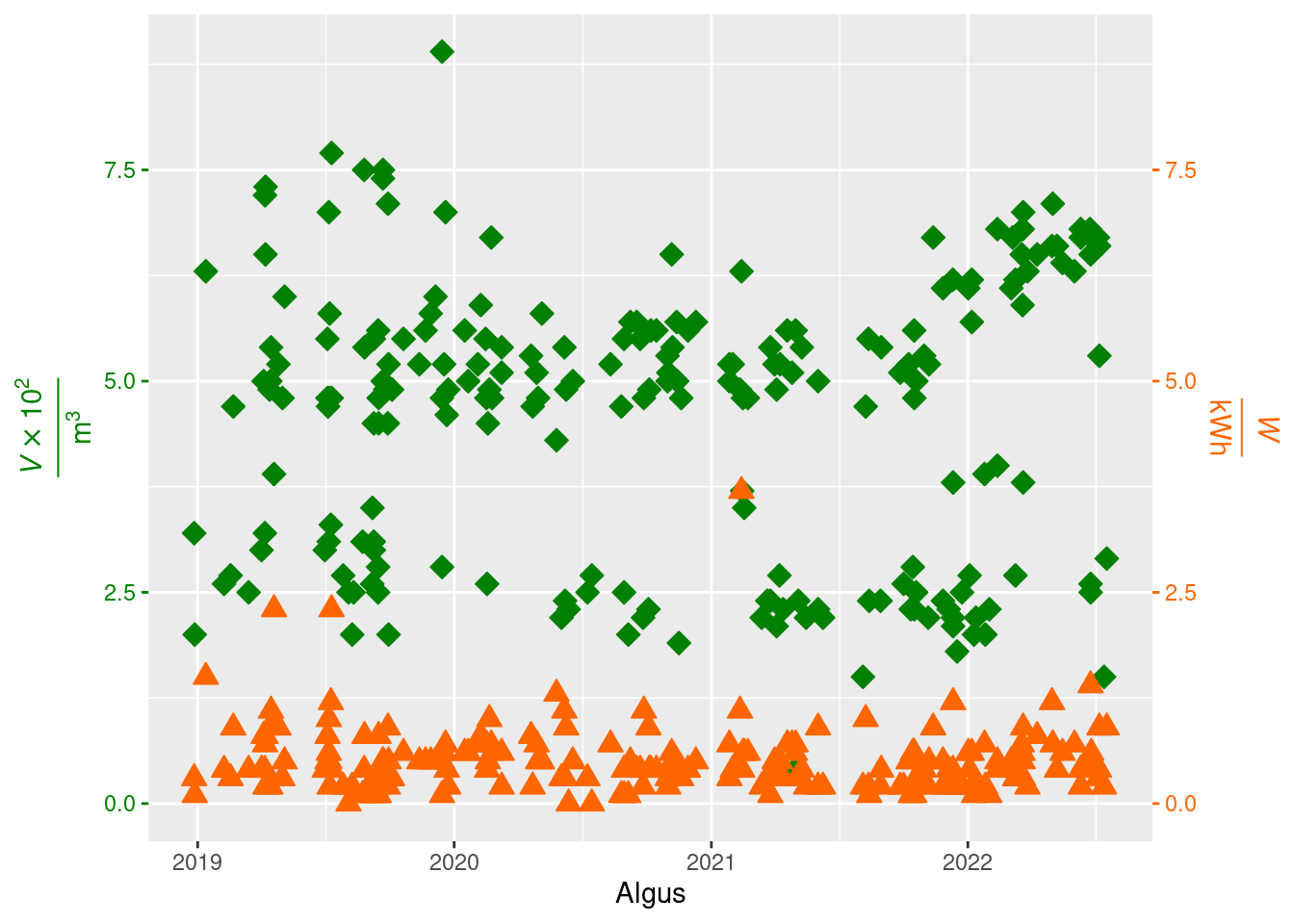
Figure 5.3: Water and electricity consumption between 2018-12-27 00:58:00 and 2022-07-17 15:33:00 .

5.14.4 Trend line

On the figure 5.4 on the page .

ggplot(data = washing_cycles_with_full_records, aes(x = `Temperatuur`, y = `Pöördeid.min`)) + geom_point(shape = 23, color = "#008000", fill = "#ff6600", size = 3) +  # 1
  labs(x = TeX("$\\frac{\\textit{t}}{\\degree C}$"), y = TeX("$\\frac{\\textit{f}}{min}$")) +                                                                          # 2
  geom_smooth()                                                                                                                                                        # 3
## `geom_smooth()` using method = 'loess' and formula
## = 'y ~ x'
## Warning in simpleLoess(y, x, w, span, degree = degree, parametric = parametric,
## : pseudoinverse used at 29.7
## Warning in simpleLoess(y, x, w, span, degree = degree, parametric = parametric,
## : neighborhood radius 10.3
## Warning in simpleLoess(y, x, w, span, degree = degree, parametric = parametric,
## : reciprocal condition number 2.4663e-30
## Warning in simpleLoess(y, x, w, span, degree = degree, parametric = parametric,
## : There are other near singularities as well. 100
## Warning in predLoess(object$y, object$x, newx = if (is.null(newdata)) object$x
## else if (is.data.frame(newdata))
## as.matrix(model.frame(delete.response(terms(object)), : pseudoinverse used at
## 29.7
## Warning in predLoess(object$y, object$x, newx = if (is.null(newdata)) object$x
## else if (is.data.frame(newdata))
## as.matrix(model.frame(delete.response(terms(object)), : neighborhood radius
## 10.3
## Warning in predLoess(object$y, object$x, newx = if (is.null(newdata)) object$x
## else if (is.data.frame(newdata))
## as.matrix(model.frame(delete.response(terms(object)), : reciprocal condition
## number 2.4663e-30
## Warning in predLoess(object$y, object$x, newx = if (is.null(newdata)) object$x
## else if (is.data.frame(newdata))
## as.matrix(model.frame(delete.response(terms(object)), : There are other near
## singularities as well. 100
Graph with a trend line.

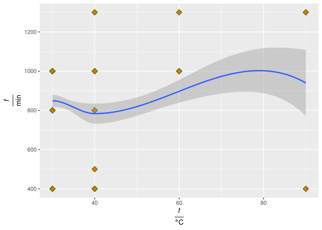
Figure 5.4: Graph with a trend line.

5.14.5 Regression and correlation

The figure 5.5 on the page represents the correlation between the water and electricity consumption between 2018-12-27 00:58:00 and 2022-07-17 15:33:00. The plot displays the smooth regression line[78] and the correlation coefficient. There are also the data about the regression. Both labels have been positioned vertically.

For ggpubr, the dependency nloptr must be installed directly in Ubuntu[79]:

sudo apt-get install libnlopt-dev  # 1
                                   # 2
librarian::shelf(c(                                                                                                                                                                                         # 1
  "ggplot2",                                                                                                                                                                                                # 2
  "ggpmisc", #for stat_poly_line                                                                                                                                                                            # 3
  "ggpubr", # for stat_regline_equation                                                                                                                                                                     # 4
  "latex2exp"                                                                                                                                                                                               # 5
))                                                                                                                                                                                                          # 6
                                                                                                                                                                                                            # 7
if (!decimal_separator_period) { # for stat_regline_equation and stat_cor                                                                                                                                   # 8
  options(OutDec = ".")                                                                                                                                                                                     # 9
}                                                                                                                                                                                                          # 10
ggplot(data = washing_cycles_with_full_records, mapping = aes(x = `Veekulu..l.`, y = `kWh`)) +                                                                                                             # 11
  geom_point(shape = 23, color = "#ff6600", fill = "#ff6600", size = 3) +                                                                                                                                  # 12
  labs(x = TeX("$\\frac{\\textit{V}}{m^3}$"), y = TeX("$\\frac{\\textit{W}}{kWh}$")) +                                                                                                                     # 13
  stat_poly_line() +                                                                                                                                                                                       # 14
  stat_regline_equation(mapping = aes(x = `Veekulu..l.`, y = `kWh`, label = paste(after_stat(eq.label), after_stat(rr.label), after_stat(adj.rr.label), sep = "~~~~")), color = "#ff6600", label.y = 3) +  # 15
  stat_cor(aes(x = `Veekulu..l.`, y = `kWh`), color = "#ff6600", label.y = 2.5)                                                                                                                            # 16
Correlation between the water and electricity consumption between 2018-12-27 00:58:00 and 2022-07-17 15:33:00 .

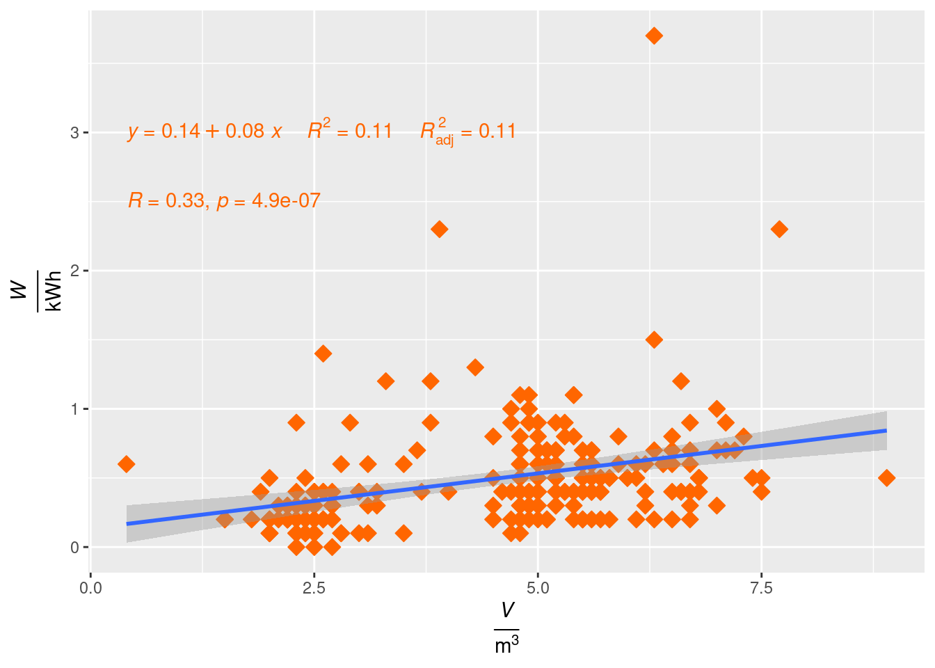
Figure 5.5: Correlation between the water and electricity consumption between 2018-12-27 00:58:00 and 2022-07-17 15:33:00 .

if (!decimal_separator_period) {  # 1
  options(OutDec = ",")           # 2
}                                 # 3

It is possible to use different kind of trend lines as seen on the figure 5.6 on the page :

omega <- c(932.0058, 827.2861, 733.0383, 628.3185, 523.5988)                      # 1
h <- c(303.44868, 239.08893, 187.71603, 137.91380,  95.77349)                     # 2
                                                                                  # 3
data_frame_of_precession_with_height_without_outliers <- data.frame(              # 4
  omega,                                                                          # 5
  h                                                                               # 6
)                                                                                 # 7
                                                                                  # 8
color_of_height <- "#ff00ff"                                                      # 9
color_x <- "#008000"                                                             # 10
                                                                                 # 11
ggplot(                                                                          # 12
  data <- data_frame_of_precession_with_height_without_outliers,                 # 13
  mapping <- aes(x = omega, y = h)                                               # 14
) +                                                                              # 15
  geom_point(shape = 23, size = 1) +                                             # 16
  labs(x = TeX("$\\frac{\\omega}{\\frac{1}{s}}$"), y = TeX("$\\frac{h}{m}$")) +  # 17
  theme(                                                                         # 18
    axis.title.x = element_text(colour = color_x),                               # 19
    axis.text.x = element_text(colour = color_x),                                # 20
    axis.ticks.x = element_line(colour = color_x),                               # 21
    axis.title.y = element_text(colour = color_of_height),                       # 22
    axis.text.y = element_text(colour = color_of_height),                        # 23
    axis.ticks.y = element_line(colour = color_of_height)                        # 24
  ) +                                                                            # 25
  stat_poly_line(formula = y ~ poly(x, 2))                                       # 26
Polynomial trend line with the degree \num{2}.

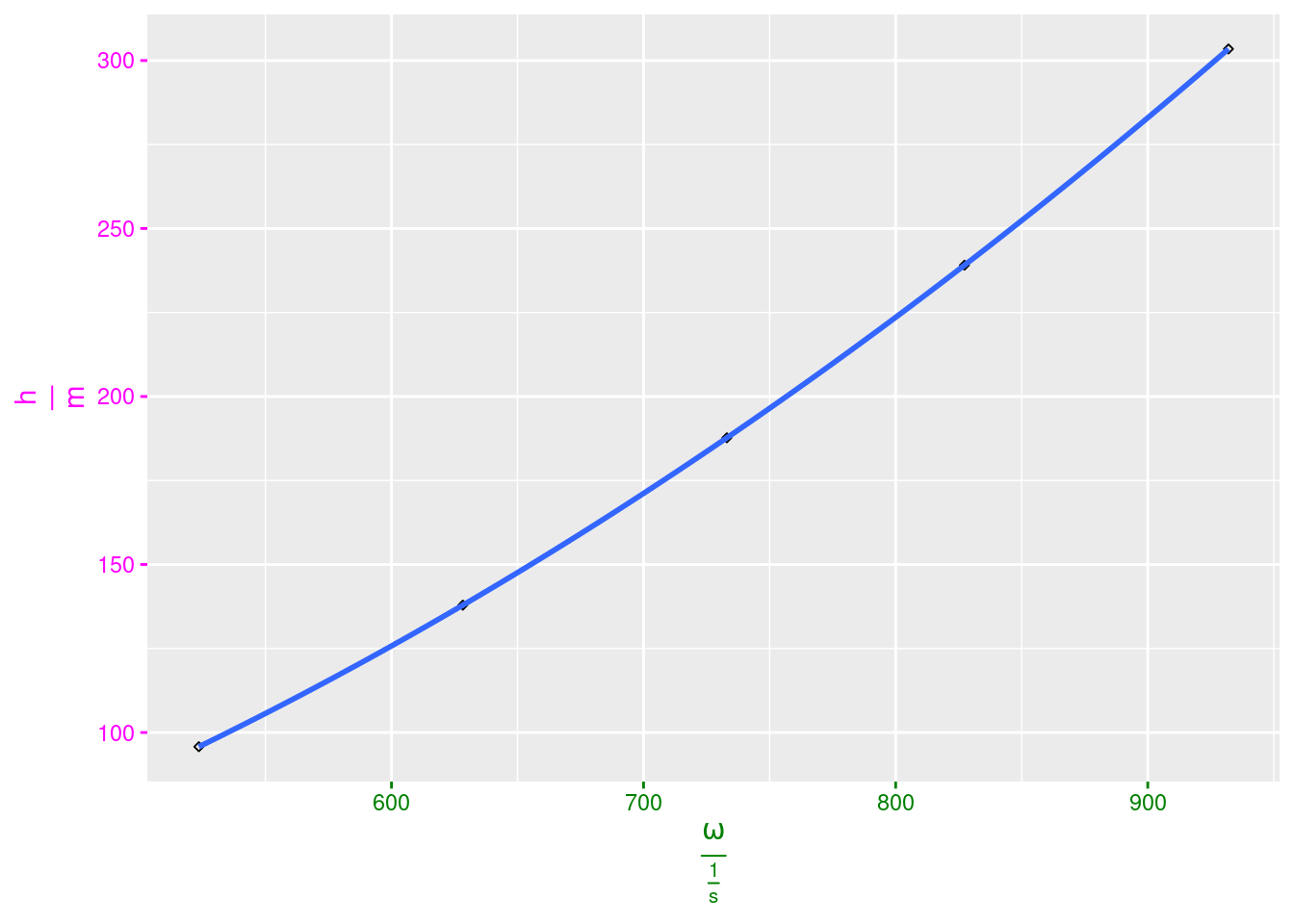
Figure 5.6: Polynomial trend line with the degree .

5.14.6 Error bars

The figure 5.7 on the page represents the water and electricity consumption between 2018-12-27 00:58:00 and 2022-07-17 15:33:00 with errorbars.

                                                                                                                                                                                                                                                                                                  # 1
librarian::shelf(c(                                                                                                                                                                                                                                                                               # 2
  "ggplot2",                                                                                                                                                                                                                                                                                      # 3
  "latex2exp"                                                                                                                                                                                                                                                                                     # 4
))                                                                                                                                                                                                                                                                                                # 5
                                                                                                                                                                                                                                                                                                  # 6
margin_of_V <- 1e-3 / 2 * 2 * 1e2                                                                                                                                                                                                                                                                 # 7
margin_of_W <- .1 / 2                                                                                                                                                                                                                                                                             # 8
                                                                                                                                                                                                                                                                                                  # 9
color_x <- "#008000"                                                                                                                                                                                                                                                                             # 10
color_y <- "#ff6600"                                                                                                                                                                                                                                                                             # 11
                                                                                                                                                                                                                                                                                                 # 12
ggplot(data = washing_cycles_with_full_records, mapping = aes(x = `veekulu_dal`, y = `kWh`)) +                                                                                                                                                                                                   # 13
  geom_point(shape = 23, size = 1) +                                                                                                                                                                                                                                                             # 14
  labs(x = TeX("$\\frac{\\textit{V} \\times 10^2}{m^3}$"), y = TeX("$\\frac{\\textit{W}}{kWh}$")) +                                                                                                                                                                                              # 15
  geom_errorbarh(aes(xmin = `veekulu_dal` - margin_of_V, xmax = `veekulu_dal` + margin_of_V, y = `kWh`), color = color_x) +                                                                                                                                                                      # 16
  geom_errorbar(aes(x = `veekulu_dal`, ymin = `kWh` - margin_of_W, ymax = `kWh` + margin_of_W), color = color_y) +                                                                                                                                                                               # 17
  theme(axis.title.x = element_text(colour = color_x), axis.text.x = element_text(colour = color_x), axis.ticks.x = element_line(colour = color_x), axis.title.y = element_text(colour = color_y), axis.text.y = element_text(colour = color_y), axis.ticks.y = element_line(colour = color_y))  # 18
Water and electricity consumption between 2018-12-27 00:58:00 and 2022-07-17 15:33:00  with errobars.

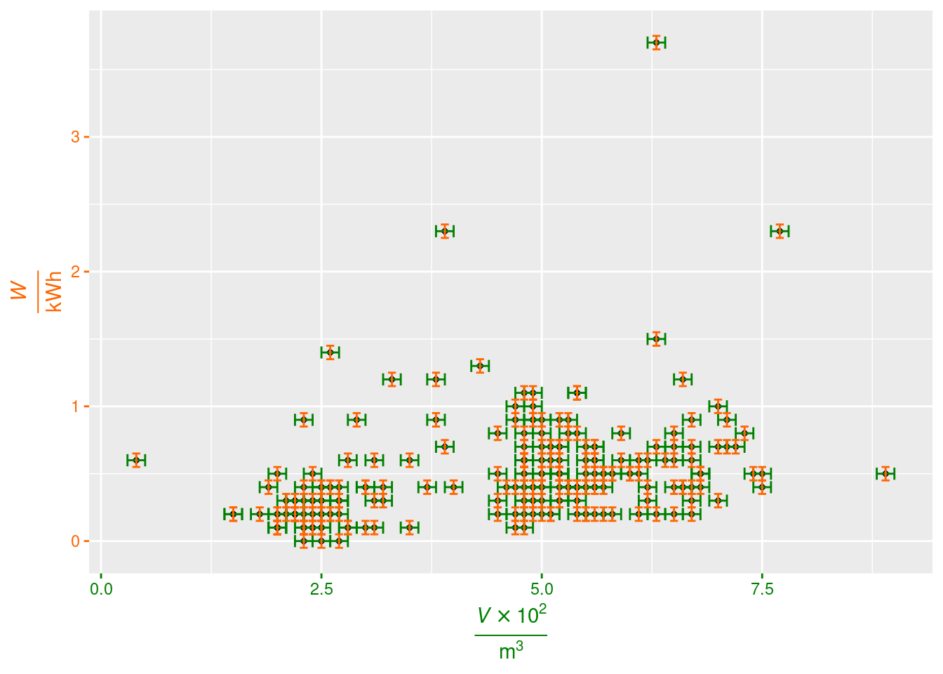
Figure 5.7: Water and electricity consumption between 2018-12-27 00:58:00 and 2022-07-17 15:33:00 with errobars.

Joonisel 5.8 leheküljel on esitatud valgustugevuse mõõtmise tulemused keskväärtuse ja mõõtemääramatustega: mustaga on tähistatud A-, oranžiga B1-, roosaga B2-tüüpi ja rohelisega kogu mõõtemääramatus[80]. Sellelt jooniselt näeme, kui palju mingit tüüpi mõõtemääramatus antud juhul mõju avaldab.

librarian::shelf(c(                                                                                                                                                     # 1
  "ggplot2",                                                                                                                                                            # 2
  "latex2exp"                                                                                                                                                           # 3
))                                                                                                                                                                      # 4
color_x <- "#008000"                                                                                                                                                    # 5
illuminance <- c(923, 905, 593, 587)                                                                                                                                    # 6
illuminance_data_frame = data.frame(illuminance)                                                                                                                        # 7
illuminance_mean <- mean(illuminance)                                                                                                                                   # 8
illuminance_se <- as.numeric(mean_se(illuminance)["ymax"] - illuminance_mean)                                                                                           # 9
illuminance_size <- length(illuminance)                                                                                                                                # 10
illuminance_size_less_1 <- illuminance_size - 1                                                                                                                        # 11
librarian::shelf(c(                                                                                                                                                    # 12
  "distributions3"                                                                                                                                                     # 13
))                                                                                                                                                                     # 14
studentTDistribution = StudentsT(df = illuminance_size_less_1)                                                                                                         # 15
alpha <- 0.05                                                                                                                                                          # 16
probability_for_Student <- 1 - alpha / 2                                                                                                                               # 17
caliper_number_student = quantile(studentTDistribution, probability_for_Student)                                                                                       # 18
illuminance_uncertainty_A <- caliper_number_student * illuminance_se                                                                                                   # 19
                                                                                                                                                                       # 20
precision_ratio <- .05                                                                                                                                                 # 21
number_of_least_sigfig = 10                                                                                                                                            # 22
student_inf <- quantile(StudentsT(df = Inf), probability_for_Student)                                                                                                  # 23
illuminance_uncertainty_B_1 <- student_inf * (illuminance_mean * precision_ratio + number_of_least_sigfig) / 3                                                         # 24
                                                                                                                                                                       # 25
illuminance_smallest_unit <- 1                                                                                                                                         # 26
probability <- 1 - alpha                                                                                                                                               # 27
                                                                                                                                                                       # 28
illuminance_uncertainty_B_2 <- probability * illuminance_smallest_unit / 2                                                                                             # 29
                                                                                                                                                                       # 30
illuminance_uncertainty <- sqrt(illuminance_uncertainty_A^2 + illuminance_uncertainty_B_1^2 + illuminance_uncertainty_B_2^2)                                           # 31
                                                                                                                                                                       # 32
ggplot(data = illuminance_data_frame, mapping = aes(x = `illuminance`, y = 0)) +                                                                                       # 33
  geom_point(shape = 23, size = 1) +                                                                                                                                   # 34
  geom_point(aes(x = illuminance_mean, y = 0), shape = 23, size = 2, color = color_x) +                                                                                # 35
  labs(x = TeX("$\\frac{\\textit{q}}{lx}$")) +                                                                                                                         # 36
  geom_errorbarh(aes(xmin = illuminance_mean - illuminance_uncertainty, xmax = illuminance_mean + illuminance_uncertainty), color = color_x) +                         # 37
  geom_errorbarh(aes(xmin = illuminance_mean - illuminance_uncertainty_A, xmax = illuminance_mean + illuminance_uncertainty_A), height = .1) +                         # 38
  geom_errorbarh(aes(xmin = illuminance_mean - illuminance_uncertainty_B_1, xmax = illuminance_mean + illuminance_uncertainty_B_1), color = "#ff6600", height = .2) +  # 39
  geom_errorbarh(aes(xmin = illuminance_mean - illuminance_uncertainty_B_2, xmax = illuminance_mean + illuminance_uncertainty_B_2), color = "#ff66ff", height = .4) +  # 40
  theme(                                                                                                                                                               # 41
    axis.title.x = element_text(colour = color_x),                                                                                                                     # 42
    axis.text.x = element_text(colour = color_x),                                                                                                                      # 43
    axis.ticks.x = element_line(colour = color_x),                                                                                                                     # 44
    axis.title.y=element_blank(),                                                                                                                                      # 45
    axis.text.y=element_blank(),                                                                                                                                       # 46
    axis.ticks.y=element_blank()                                                                                                                                       # 47
  )                                                                                                                                                                    # 48
## Warning in geom_point(aes(x = illuminance_mean, y = 0), shape = 23, size = 2, : All aesthetics have length 1, but the data has 4
## rows.
## ℹ Please consider using `annotate()` or provide
##   this layer with data containing a single row.
Valgustugevus koos keskmise valgustugevuse ja mõõtemääramatustega.

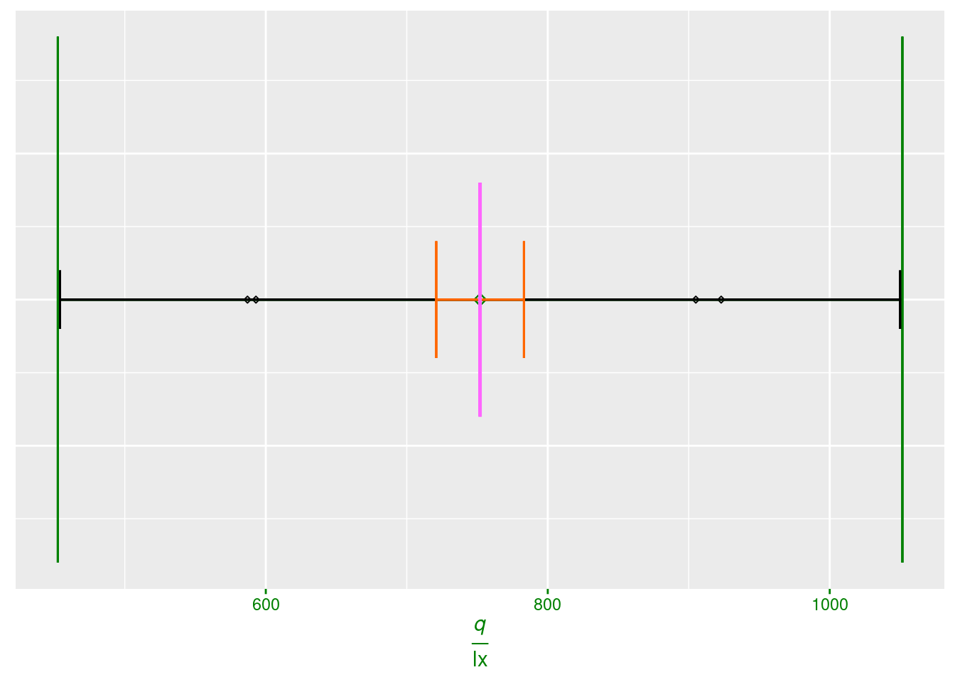
Figure 5.8: Valgustugevus koos keskmise valgustugevuse ja mõõtemääramatustega.

5.14.7 Accuracy

Joonisel 5.9 leheküljel on esitatud mõõdetud keskväärtus koos mõõtemääramatusega graafiliselt.

librarian::shelf(c(                                                                                                                                    # 1
  "ggplot2",                                                                                                                                           # 2
  "latex2exp"                                                                                                                                          # 3
))                                                                                                                                                     # 4
                                                                                                                                                       # 5
color_x <- "#008000"                                                                                                                                   # 6
ruler_smallest_unit <- .5                                                                                                                              # 7
ruler_relation = 4000 / 400                                                                                                                            # 8
ruler_smallest_unit_actual <- ruler_smallest_unit * ruler_relation                                                                                     # 9
ruler_x <- 42                                                                                                                                         # 10
ruler_x_actual <- ruler_x * ruler_relation                                                                                                            # 11
ruler_data_frame <- data.frame(ruler_x_actual)                                                                                                        # 12
                                                                                                                                                      # 13
plot <- ggplot(data = ruler_data_frame, mapping = aes(x = `ruler_x_actual`, y = 0)) +                                                                 # 14
  geom_point(shape = 23, size = 1) +                                                                                                                  # 15
  labs(x = TeX("$\\frac{\\textit{q}}{m}$")) +                                                                                                         # 16
  geom_errorbarh(aes(xmin = `ruler_x_actual` - ruler_smallest_unit_actual, xmax = `ruler_x_actual` + ruler_smallest_unit_actual), color = color_x) +  # 17
  theme(                                                                                                                                              # 18
    axis.title.x = element_text(colour = color_x),                                                                                                    # 19
    axis.text.x = element_text(colour = color_x),                                                                                                     # 20
    axis.ticks.x = element_line(colour = color_x),                                                                                                    # 21
    axis.title.y=element_blank(),                                                                                                                     # 22
    axis.text.y=element_blank(),                                                                                                                      # 23
    axis.ticks.y=element_blank()                                                                                                                      # 24
  )                                                                                                                                                   # 25
                                                                                                                                                      # 26
plot                                                                                                                                                  # 27
Kahe kontrollpunkti omavaheline kaugus mõõtemääramatusega.

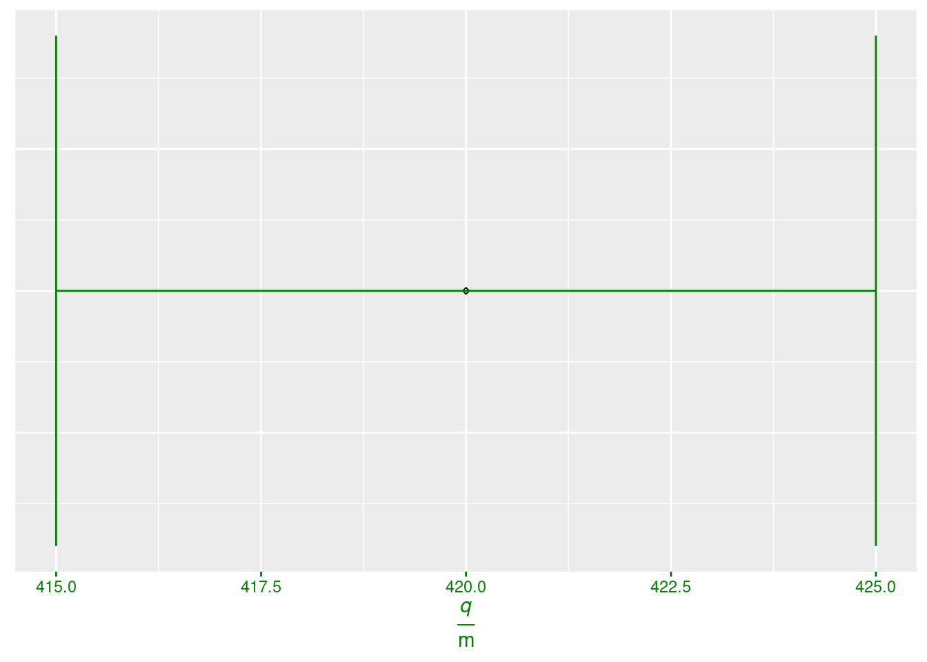
Figure 5.9: Kahe kontrollpunkti omavaheline kaugus mõõtemääramatusega.

The figure 5.10 on the page shows how to specify the accuracy of the numbers on axis[34].

plot +                                           # 1
  scale_x_continuous(                            # 2
    labels = scales::label_number(accuracy = 1)  # 3
  )                                              # 4
With specified accuracy.

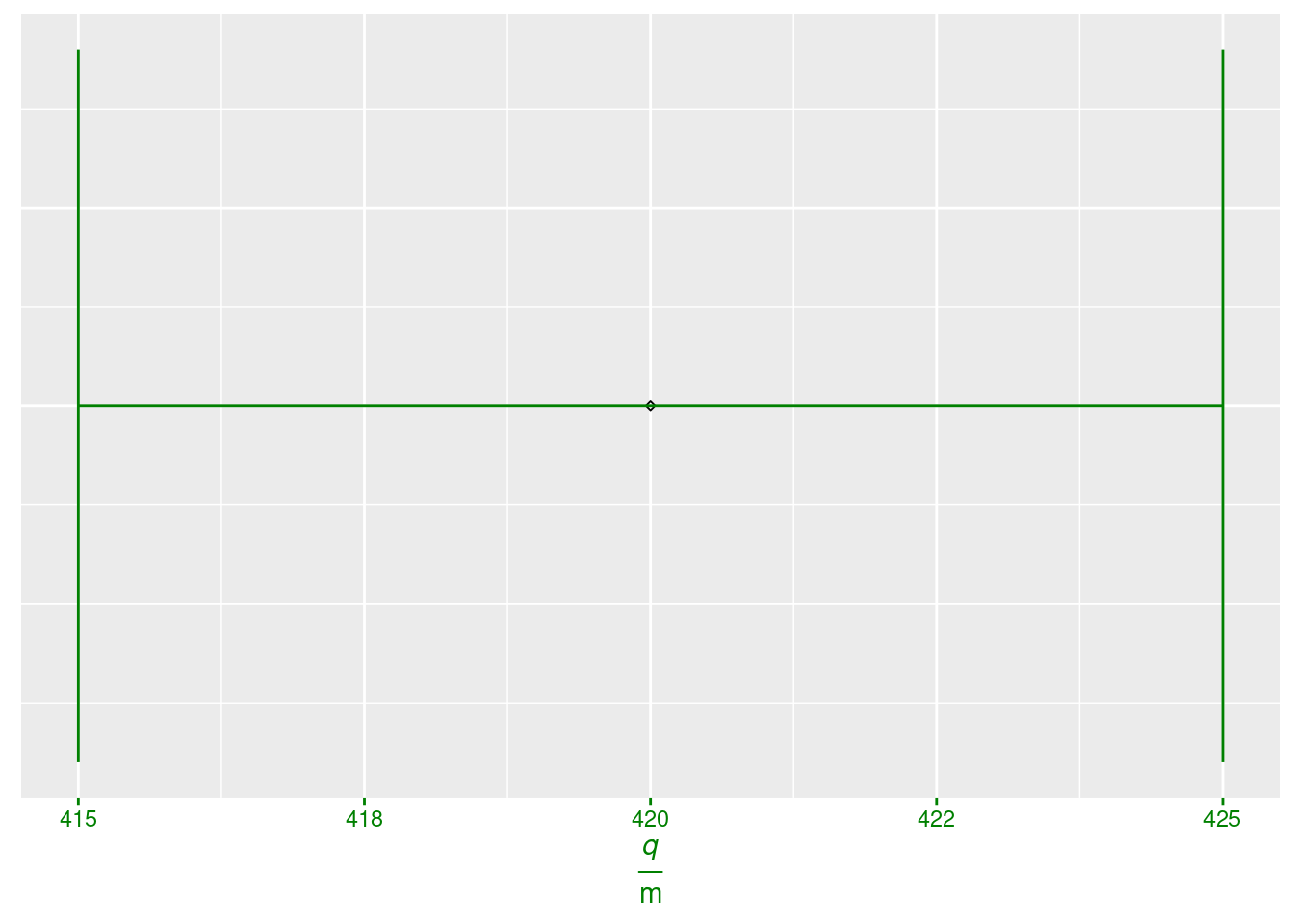
Figure 5.10: With specified accuracy.

5.15 Regression model[81]

angular_acceleration <- c(5.902952, 17.246897, 28.401369, 38.892302, 45.907424)  # 1
torque <- c(0.001153365, 0.002174215, 0.003190228, 0.004201956, 0.005009516)     # 2
formula = torque ~ angular_acceleration                                          # 3
model = lm(formula = formula)                                                    # 4
                                                                                 # 5
b <- model$coefficients[1]                                                       # 6
k <- model$coefficients[2]                                                       # 7
Regressioonisirge tõus on \qty{`r as.character(signif(x = k, digits = 3))`}{\kg\m\squared} ja see näitab inertsimomenti. Vabaliige on \qty{`r as.character(signif(x = b, digits = 3))`}{\N\m} ja see näitab hõõrdejõu momenti.  # 1
                                                                                                                                                                                                                                # 2

Regressioonisirge tõus on ja see näitab inertsimomenti. Vabaliige on ja see näitab hõõrdejõu momenti.

5.16 Correlation

In order to get the values of the result of a correlation analysis, one can use cor[82].

cor(                                               # 1
  washing_cycles_with_full_records$`Veekulu..l.`,  # 2
  washing_cycles_with_full_records$`kWh`,          # 3
  method = 'pearson'                               # 4
)                                                  # 5
## [1] 0.3320582

5.17 Linearizing

Lasen joonestada pretsessiooninurkkiiruse sõltuvuse graafiku rootori osakeste nurkkiirusest (joonis 5.11 leheküljel ).

librarian::shelf(c(                                                                                                                                                        # 1
  "ggplot2",                                                                                                                                                               # 2
  "latex2exp"                                                                                                                                                              # 3
))                                                                                                                                                                         # 4
                                                                                                                                                                           # 5
color_x <- "#008000"                                                                                                                                                       # 6
color_y <- "#ff6600"                                                                                                                                                       # 7
                                                                                                                                                                           # 8
number_of_rows_in_data_frame_of_precession <- nrow(data_frame_of_precession)                                                                                               # 9
data_frame_of_precession_without_outliers <- data_frame_of_precession[-c((number_of_rows_in_data_frame_of_precession - 1):number_of_rows_in_data_frame_of_precession), ]  # 10
                                                                                                                                                                          # 11
ggplot(                                                                                                                                                                   # 12
  data <- data_frame_of_precession_without_outliers,                                                                                                                      # 13
  mapping <- aes(x = `$\\frac{\\omega}{\\unit{\\per\\s}}$`, y = `$\\frac{\\omega_\\text{P}}{\\unit{\\per\\s}}$`)                                                          # 14
) +                                                                                                                                                                       # 15
  geom_point(shape = 23, size = 1) +                                                                                                                                      # 16
  labs(x = TeX("$\\frac{\\omega}{\\frac{1}{s}}$"), y = TeX("$\\frac{\\omega_P}{\\frac{1}{s}}$")) +                                                                        # 17
  theme(                                                                                                                                                                  # 18
    axis.title.x = element_text(colour = color_x),                                                                                                                        # 19
    axis.text.x = element_text(colour = color_x),                                                                                                                         # 20
    axis.ticks.x = element_line(colour = color_x),                                                                                                                        # 21
    axis.title.y = element_text(colour = color_y),                                                                                                                        # 22
    axis.text.y = element_text(colour = color_y),                                                                                                                         # 23
    axis.ticks.y = element_line(colour = color_y)                                                                                                                         # 24
  )                                                                                                                                                                       # 25
Pretsessiooninurkkiiruse sõltuvus rootori osakeste nurkkiirusest.

Figure 5.11: Pretsessiooninurkkiiruse sõltuvus rootori osakeste nurkkiirusest.

Teooria seosega (5.1) leheküljel ennustab pöördvõrdelist sõltuvust.

\[\begin{align} \omega_\text{P} = \frac{((\overrightarrow{r_\text{balancer; final}} - \overrightarrow{r_\text{balancer; initial}})) \times \overrightarrow{F_\text{balancer}}}{I \cdot \vec{\omega}}. \tag{5.1} \end{align}\]

Joonisel 5.11 leheküljel olev graafik lineariseeritud kujul[83] on esitatud joonisel 5.12 leheküljel .

data_frame_of_precession_without_outliers_linearized <- mutate(.data = data_frame_of_precession_without_outliers, linearized_omega = 1 / `$\\frac{\\omega}{\\unit{\\per\\s}}$`, .keep = "unused", .after = `$\\frac{\\omega}{\\unit{\\per\\s}}$`)  # 1
colnames(data_frame_of_precession_without_outliers_linearized) <- c(                                                                                                                                                                               # 2
  "$\\frac{\\frac{1}{\\omega}}{\\unit{\\s}}$",                                                                                                                                                                                                     # 3
  "$\\frac{\\omega_\\text{P}}{\\unit{\\per\\s}}$"                                                                                                                                                                                                  # 4
)                                                                                                                                                                                                                                                  # 5
                                                                                                                                                                                                                                                   # 6
ggplot(                                                                                                                                                                                                                                            # 7
  data <- data_frame_of_precession_without_outliers_linearized,                                                                                                                                                                                    # 8
  mapping <- aes(x = `$\\frac{\\frac{1}{\\omega}}{\\unit{\\s}}$`, y = `$\\frac{\\omega_\\text{P}}{\\unit{\\per\\s}}$`)                                                                                                                             # 9
) +                                                                                                                                                                                                                                               # 10
  geom_point(shape = 23, size = 1) +                                                                                                                                                                                                              # 11
  labs(x = TeX("$\\frac{\\frac{1}{\\omega}}{s}$"), y = TeX("$\\frac{\\omega_P}{\\frac{1}{s}}$")) +                                                                                                                                                # 12
  theme(                                                                                                                                                                                                                                          # 13
    axis.title.x = element_text(colour = color_x),                                                                                                                                                                                                # 14
    axis.text.x = element_text(colour = color_x),                                                                                                                                                                                                 # 15
    axis.ticks.x = element_line(colour = color_x),                                                                                                                                                                                                # 16
    axis.title.y = element_text(colour = color_y),                                                                                                                                                                                                # 17
    axis.text.y = element_text(colour = color_y),                                                                                                                                                                                                 # 18
    axis.ticks.y = element_line(colour = color_y)                                                                                                                                                                                                 # 19
  )                                                                                                                                                                                                                                               # 20
Lineariseeritud nurkkiiruste graafik. Propelleri nurkkiiruse asemel on esitatud selle pöördväärtus, mis näitab, mitu sekundit ühe radiaani läbimine kestis.

Figure 5.12: Lineariseeritud nurkkiiruste graafik. Propelleri nurkkiiruse asemel on esitatud selle pöördväärtus, mis näitab, mitu sekundit ühe radiaani läbimine kestis.

5.18 Embedding

Including works for web output[84]:

if (knitr::is_html_output()) {                               # 1
  knitr::include_url("https://learningapps.org/view409713")  # 2
}                                                            # 3
                                                             # 4

5.19 Figures

5.19.1 Displaying a figure

For figures, i created a wrapper function include_external_graphics() for knitr’s include_graphics() because natively, include_graphics() doesn’t support all the necessary file types:

```{r label = "<label of figure>", echo=FALSE, fig.cap = "<caption of figure>"}  # 1
include_external_graphics("<path-to-image-file>")                                # 2
                                                                                 # 3
```                                                                              # 4
                                                                                 # 5

For this code chunk, i use the label and the following options:

label
the label that can be referenced must not include underscores but can include dashes
fig.cap
the caption of the figure. This must be present in order to reference it.

Other options are possible:

fig.align
i set it to have the value center if i want the image to reside in center
fig.fullheight
i set it to TRUE if the image would be printed out smaller otherwise
out.width
the width. Sometimes, the image is too wide for the page. Here, i set the width to be .92 of the height of the text part on the page as that image is rotated at a right angle: .92\\textheight
out.height
sometimes, especially images with full size tend to be still a bit too large, so i set this parameter to have a value like 96%
out.extra:
for instance to turn the image with angle that has a value in degrees

5.19.2 Referencing a figure

Referencing a figure takes place using \@ref(fig:<label of figure>).

As an example, i refer to the figure 5.13.

include_external_graphics("rmd/workflow.png")  # 1
The workflow from the written markdown to the ready output using *bookdown*.

Figure 5.13: The workflow from the written markdown to the ready output using bookdown.

5.19.3 Involving an external reference in the figure caption

If i want to include an external reference inside the figure caption, i had to use the function render_with_emojis inside the caption:

                                                                                                                                                                                     # 1
```{r label = "workflow", fig.cap = paste("The workflow from the written markdown to the ready output using *bookdown*", render_with_emojis("((ref:riederer-21))"), ".", sep = "")}  # 2
include_external_graphics("rmd/workflow.png")                                                                                                                                        # 3
                                                                                                                                                                                     # 4
```                                                                                                                                                                                  # 5
                                                                                                                                                                                     # 6

This is also obsolete because of numeric referencing.

include_external_graphics("rmd/workflow.png")  # 1
The workflow from the written markdown to the ready output using *bookdown*\fontspec{Symbola}((ref:riederer-21))\fontspec{DejaVu Serif}{}.

Figure 5.14: The workflow from the written markdown to the ready output using bookdown((ref:riederer-21)).

Here, the function paste comes handy. paste glues strings together that can be fed into that function. The last parameter is sep which can be used to set the separator between the strings. Currently, i told the function to use an empty string as a separator.

5.19.4 Subfigures

Sometimes, it would be wasting having each figure below each other if they are narrow. In such a case, I want the images to be side by side. For that, I need to involve subfig as a dependency for the print output[85]:

bookdown::pdf_book:             # 1
  extra_dependencies: "subfig"  # 2
                                # 3

Pildil 5.15 leheküljel kujutatud konteinerid sisaldavad kas segu, ühte ühendit, ühte elementi või nende kombinatsiooni. Sinised sfäärid tähistavad ühe elemendi aatomeid, rohelised sfäärid teise elemendi aatomeid.

include_external_graphics("rmd/alused-kordamine-ühendid-segu-element.svg")  # 1
include_external_graphics("rmd/alused-ühendid-element.svg")                 # 2
Konteinerid.Konteinerid.

Figure 5.15: Konteinerid.

As you see, there is no spacing between subfigures. I have not found a solution for that.

5.20 Quick-response code[86]

The example (39) with the listing ?? on the page and the figure5.16 on the page shows how to generate a quick-response code[87,88].

Newtoni kolmas seadus - viide.

Figure 5.16: Newtoni kolmas seadus - viide.